Predictive AI Development: Forecasting Model Capabilities Before Full-Scale Training

Yinusa Yakubu Temitope · Oct 20, 2026

Abstract

This proposal asks whether the probability that a model reaches a defined capability threshold can be forecast from its training configuration and cheap preliminary experiments, accurately enough to change how a fixed compute budget is spent.

Scaling laws already predict training loss well. Predicting a specific downstream capability is harder, because the mapping from loss to task performance is nonlinear, noisy across random seeds, and sensitive to how the task is measured. Recent work has made progress on this problem, so the contribution here is narrower: forecasts stated as probabilities of crossing a threshold, validated on held-out configurations, and judged by whether they reduce the total cost of reaching a target.

The programme starts with a synthetic rule-learning pilot, where generalisation can appear abruptly, then moves to code generation verified by unit tests. It fits predictors on small and early-stopped runs, records forecasts before the target runs are trained, and scores them on accuracy, calibration, and decision value against established baselines.

1. The research problem

The relationship between a training configuration and the capabilities of the resulting model is only partly characterised. Developers choose an architecture, a data mixture, an optimiser, a schedule and a compute budget, then pay the full cost of training before learning whether the model can do the task they care about.

Some of this is already predictable. Neural scaling laws describe how pretraining loss falls with parameters, data and compute, and they have guided compute allocation since Kaplan et al. (2020) and Hoffmann et al. (2022). Loss, however, is not a capability. A model can improve its average loss while its score on a specific task barely moves, and a task score can appear to jump at a scale threshold.

Predictive AI development is the study of whether a model's eventual capabilities can be forecast from its development conditions early enough to improve training decisions. The strong form of the question is probabilistic: under configuration κ, what is the probability that capability j reaches threshold c*, accounting for stochastic optimisation and run-to-run variation?

The motivation is resource allocation. If inexpensive experiments reliably predict the outcomes of expensive ones, a developer can select configurations with a higher probability of reaching a target within a given budget, and stop pursuing configurations that will not.

This is a hypothesis, not an established general capability. Its feasibility must be tested separately for each task, architecture, data regime and training procedure.

Core research question. To what extent can a model's capability profile, and its uncertainty, be predicted from architecture, training data, initialisation, objective, optimisation procedure, compute and training duration before the full training run is completed?

Applied research question. Can those predictions allocate compute, data, engineering effort and training time better than scaling-based planning and empirical trial and error?

Sub-questions.

1. RQ1: Which development variables predict the selected capability?
2. RQ2: How stable are those relationships across seeds and training histories?
3. RQ3: Does the predictor generalise to configurations it has not seen?
4. RQ4: Does prediction-guided allocation outperform baseline allocation?
5. RQ5: How well does the framework quantify its uncertainty and flag settings where it should not be trusted?

Primary hypothesis. For a defined family of models and tasks, measurable properties of the development process carry enough information to forecast selected capability outcomes, and their uncertainty, on unseen training configurations better than simple baselines.

Secondary hypotheses. Each is tested in the section named.

• H1. Capability outcomes vary systematically with initialisation, data order, data composition, optimisation choices, training duration and compute (Sections 4 and 5).
• H2. Variation in final weights is not a sufficient proxy for variation in capability; behaviour, and where feasible internal mechanisms, must be measured directly (Section 4).
• H3. Small-scale experiments carry predictive signal about larger scales, but transfer is tested, not assumed (Section 5, extrapolation ratio ρ).
• H4. Prediction-guided allocation lowers the cost of reaching a target capability profile relative to a defined baseline process (Section 7).
• H5. A useful predictor quantifies its uncertainty and identifies where its forecasts are unreliable (Section 6).

The initial study targets one narrow, measurable capability family. Predicting every capability of arbitrary systems, or deriving a complete theory of intelligence, is a long-term ambition and not a first experiment.

2. Formal setup

The forecasting target is a probability distribution over a measured capability, conditioned on a configuration and on whatever information exists at the moment the forecast is made.

Configuration and randomness. A training configuration collects the choices a developer controls. Random seeds are kept separate, because they are not choices in the same sense and their effect must be estimated, not optimised.

Training is then a stochastic map from configuration and seed to weights, and training compute for a dense transformer is approximately six FLOPs per parameter per token.

The components of κ are not independent. Tokens processed depend on compute and model size, and the best learning rate shifts with model size and batch size. The design in Section 5 has to respect these couplings.

Capability. Capability j is defined by an evaluation distribution $P_{j}$ and a per-item score $m_{j}$ (for example, 1 if generated code passes all unit tests). The true capability is an expectation; what we observe is a finite-sample estimate on n items.

Information sets. A forecast is only meaningful relative to what was known when it was made. Let H be the record of completed pilot runs and $O_{≤t}$ the measurements from the target run up to step t (losses, gradient statistics, intermediate evaluations).

A forecast made with $I_{0}$ is an ex ante forecast from configuration and pilots. A forecast made with $I_{t}$ for t > 0 is an in-run forecast. They answer different questions and must be reported separately; a method that needs early-run measurements cannot be described as predicting from configuration alone.

The forecasting object. The predictor returns a predictive distribution, not a point. From it we read the point forecast, an interval, and the quantity that matters for decisions: the probability of crossing the threshold.

The probability is taken over both the unknown seed s and the predictor's own uncertainty about the configuration's mean outcome.

Capability profile. A model is rarely judged on one capability. The profile collects every measured ability and operating property that matters for the intended use, such as task accuracy, reliability across seeds, latency, memory, robustness under distribution shift, and safety evaluations.

Sections 3 to 6 develop the method for a single component $Y_{j}$. Section 7 returns to the full profile, because capabilities can trade off against one another and the allocation decision depends on all of them.

Symbol	Meaning
κ	Training configuration: architecture A, data mixture D, optimiser and hyperparameters O, parameters N, training tokens T
s	Random seed: initialisation and data order
w	Trained weights
$F_{\text{train}}$	Training compute in FLOPs
L	Held-out pretraining loss
$Y_{j}$	True capability on task j
$Ŷ_{j}$	Measured capability on n evaluation items
$y^{*}_{j}$	Capability threshold that counts as success
$I_{t}$	Information available at forecast point t
$\hat{π}_{j}$(κ)	Forecast probability that κ reaches $y^{*}_{j}$
K, B	Development cost, available budget

3. Why capability prediction is harder than loss prediction

Loss is smooth in scale; capability is a nonlinear, noisy and resolution-limited function of loss. Each of those three properties adds error that a loss forecast does not have.

Stage one: loss is predictable. For a fixed architecture family and data distribution, held-out loss is well described by a parametric law in parameters N and tokens T, with an irreducible term E (Hoffmann et al., 2022).

The constants are fitted on small runs and the law is extrapolated. This works when the data distribution and training recipe stay fixed, and degrades when they change.

Stage two: the link from loss to capability is nonlinear. Task performance is commonly modelled as a function of loss. A logistic link captures the common pattern: a floor near chance, a steep middle, and a ceiling.

Here σ is the logistic function, $L_{0,j}$ is the loss at which task j is halfway between floor and ceiling, and $k_{j}$ sets how sharp the transition is. Other functional forms are used in the literature; the logistic is a working assumption to be tested, not a result.

Why the steep middle is the hard part. Composing the two stages propagates loss error into capability error. A first-order approximation makes the mechanism explicit.

The slope is largest exactly where the capability transitions, so a small error in the forecast loss becomes a large error in forecast capability at the point where the decision matters most. This is a precise statement of why apparent emergence is difficult to forecast, and why two-stage methods can compound errors. Krajewski et al. argue for modelling downstream accuracy directly from training budget for this reason; whether direct or two-stage forecasting extrapolates better is itself an empirical question for this programme.

Resolution. A capability measured on n items has sampling error, and a pass rate below roughly 1/n is invisible. Sampling k completions per item lowers the floor.

Hu et al. (2024) pushed this to its limit with PassUntil, which samples until a first success and so measures very small pass probabilities in small models. With that resolution they found task performance followed a smooth scaling relation, and they forecast the code-generation performance of a 2.4B-parameter model before training it. The general lesson: some apparent discontinuities are measurement artefacts, and the evaluation protocol is part of the forecasting method.

Three targets. A predictive method must state which of these it forecasts.

1. Training dynamics: loss and optimisation behaviour during training.
2. Task performance: $Y_{j}$ on a fixed evaluation distribution $P_{j}$.
3. Capability: reliable performance on a defined class of tasks, including held-out variants that test generalisation rather than benchmark-specific fit.

The third target needs more than one evaluation. A benchmark score is evidence about one distribution, so claims about capability should be backed by tests for memorisation, distribution sensitivity and contamination.

4. Stochasticity and measurement noise

Two models trained from the same configuration with different seeds can land on different capabilities, so a configuration does not have one outcome; it has a distribution of outcomes. Forecasts must target that distribution.

Where run-to-run variation comes from. Training is a deterministic procedure once every input is fixed. Two runs with the same initialisation, data order, software and deterministic kernels should ordinarily produce the same weights. Variation enters through the seed (initialisation and data order), through non-deterministic GPU operations and reduction order, and through differences in software versions and hardware. The experiments log all of these, and a first control run confirms that fixing them does reproduce the result.

Three levels of difference. Two runs can differ at three levels, and they must be measured separately because one does not imply another.

1. Parameters. The weights differ. Networks have many symmetries (for example, permuting hidden units), so different weights can implement the same function.
2. Behaviour. Measured capabilities differ: held-out accuracy, robustness, calibration and failure modes.
3. Mechanism. The internal representations or circuits that produce the behaviour differ, as measured with interpretability methods where the question requires it.

The forecasting target in this programme is behaviour. Weight distance is recorded but not used as a proxy for capability, which is hypothesis H2. Mechanistic measurements are added only when a forecast fails and the failure needs explaining.

A three-level model. Measured capability is the configuration's mean, plus seed variation, plus evaluation noise.

The seed variance τ² is allowed to depend on κ, because some configurations are less stable than others. For bounded scores such as pass rates, the same structure is better fitted on the logit scale or with a beta-binomial likelihood; the normal form is shown for clarity.

Variance decomposition. Across a set of runs, total observed variance splits into what the configuration explains, what the seed adds, and what the evaluation adds.

Only the first term can be predicted from κ. If seed variance dominates, the best possible ex ante forecast is still wide, and the honest output is a probability, not a number.

Threshold probability. If the predictor's estimate of the configuration mean is itself uncertain, with estimate m̂ and variance v̂, the forecast probability of reaching the threshold combines both sources.

Φ is the standard normal cumulative distribution. The threshold applies to true capability $Y_{j}$; if success is judged on the measured score, σ²_eval is added under the square root.

How many seeds. To estimate a configuration's mean within ±δ at roughly 95% confidence, the number of seeds R must satisfy the usual sample-size bound.

$τ_{j}$ is unknown in advance, so the first experiment fixes every setting except the seed and runs enough replicates to estimate it. Later experiments vary data order, training duration and data mixture, and a hierarchical model separates their effects. Seed sensitivity is well documented in smaller models, for example in the MultiBERTs reproductions; how large it is at the threshold of a target capability is the open measurement.

A forecasting method that holds for one seed or one narrow configuration has limited value. Results must report the range of conditions over which forecasts stayed accurate.

5. A controlled experimental programme

The programme starts with a pilot small enough to run many controlled replicates, then moves to a realistic task only after the pilot replicates.

Pilot: predicting generalisation on a synthetic rule. Training data is generated from a known rule, such as modular arithmetic, with held-out examples kept separate. Small networks on such tasks can fit the training set long before they generalise, and then generalise abruptly (Power et al., 2022). That makes the threshold event sharp and the forecasting problem hard in the right way, at low cost. The factors varied are seed, number and diversity of examples, model size, optimiser settings, training duration and compute, in a factorial design. The forecast targets are final held-out accuracy and the probability of crossing a predefined generalisation threshold, from configuration variables and early-training signals, recorded before outcomes are known. The pilot succeeds if the predictor shows positive skill on held-out configurations and selects a configuration that reaches the threshold at lower expected cost.

Second stage: a realistic task. Code generation verified by unit tests keeps an objective evaluation while moving to language models, where the literature in Section 9 provides strong baselines.

Success on a synthetic task is a narrow proof of concept, not a theory of large language models. Transfer to more complex tasks and architectures is what the second stage tests.

Splitting configurations. The configuration set is divided before any training into a fitting set and a held-out test set. The test set is placed beyond the fitting set in compute, so every test forecast is an extrapolation.

The extrapolation ratio ρ is reported for every result. A method that is accurate at ρ = 2 and fails at ρ = 20 has a known range, which is useful; a method reported without ρ is not.

The five stages.

1. Define the target. Fix the task, the evaluation distribution $P_{j}$, the score $m_{j}$, the threshold $y^{*}_{j}$ and the number of evaluation items n before any training. For code generation, use held-out problems with executable tests, not subjective ratings.
2. Build controlled configurations. Choose a model family and vary one factor at a time first (model size, training tokens, data mixture, seed), then use a factorial design to measure interactions. Log the full configuration, compute spent, and every evaluation.
3. Fit predictors on $K_{\text{fit}}$. Train small models and early-stopped runs. Fit candidate predictors: the two-stage loss-then-link method, a direct budget-to-capability law, and a learned predictor using early-run signals. Each is compared with simple baselines, including learning-curve extrapolation, the historical average of past runs, and the standard practice of running a few pilots and keeping the best.
4. Forecast before observing. For each configuration in $K_{\text{test}}$, record the full predictive distribution, the threshold probability $\hat{π}_{j}$ and the method used, and timestamp them before those runs begin. This blocks post hoc adjustment from being mistaken for predictive skill.
5. Train and score $K_{\text{test}}$. Train the held-out configurations across R seeds and score the recorded forecasts with the metrics in Section 6.

A final transfer test changes more than one factor at once (a new data mixture at a new scale, or a second model family) to find where forecasts break.

The criterion that matters is out-of-sample performance. A function that fits the observed runs closely but fails on unseen configurations is not a basis for spending decisions.

6. Evaluating forecasts

A forecast is scored on three things: how close it was, whether its stated uncertainty was honest, and whether it beat a simpler method. Each held-out run m contributes one realised outcome against its recorded forecast; M is the number of held-out runs.

Accuracy. Mean absolute error between the point forecast and the realised capability.

Calibration of intervals. The share of realised outcomes that fall inside the forecast 90% intervals. A calibrated method scores close to 0.90; well below means overconfident, well above means intervals are wider than they need to be.

Calibration of threshold probabilities. The Brier score measures the threshold forecasts directly. Lower is better, and a forecaster that always says 0.5 scores 0.25.

Forecasts are also grouped into probability bins (for example 0 to 0.2, 0.2 to 0.4) and the observed success rate in each bin is compared with the forecast. A reliability plot of the two is the standard visual check.

Skill against baselines. Every metric is reported relative to a baseline, so that a good number on an easy problem is not mistaken for a good method.

S is any of the error scores above. Skill above zero means the method beats the baseline; the baselines are learning-curve extrapolation, the two-stage loss method, a direct budget-to-capability scaling law, a parameter-count or compute heuristic, and running a few pilots and keeping the best.

7. From forecasting to resource allocation

The economic test is whether forecasts lower the expected cost of reaching a capability target, after paying for the forecasting itself.

The decision problem. Choose the configuration with the highest forecast probability of success, subject to a budget that includes the pilot experiments used to make the forecast.

The equivalent cost-minimising form is often more natural for a team with a fixed target: find the cheapest configuration that succeeds with probability at least 1 − δ.

Optimising a capability profile. With the full profile Y, the objective is a task-specific utility U that weighs accuracy, reliability, latency, memory, robustness and safety. Because the outcome is uncertain, the developer maximises expected utility and can bound the downside.

The single-capability problem above is the special case U = 1[$Y_{j}$ ≥ $y^{*}_{j}$], whose expectation is exactly $π_{j}$(κ). The general form matters because the goal is rarely the most capable model. It is the right profile for a task, within budget, latency, memory, reliability and deployment constraints.

Why reliability belongs in the objective. If a failed run is simply retried with a new seed, the number of runs until first success is geometric, so expected cost is the cost per run divided by the success probability.

A configuration costing 1.0 units with π = 0.3 has expected cost 3.3 units. One costing 1.5 units with π = 0.9 has expected cost 1.7 units. The cheaper run is the more expensive choice, and only a probability forecast reveals it.

The cost function. K(κ) should include more than accelerator compute where relevant: data acquisition and preparation, engineering time, evaluation, failed runs, and the inference cost of deploying the resulting model. The right accounting depends on the application.

The value of forecasting. Forecasting earns its place only if the expected saving exceeds the cost of the pilots that produce it.

Marginal value of each resource. For each resource r (compute, data, training time, engineering effort), the marginal value is the expected utility gained from one more unit, estimated by finite differences between nearby configurations.

Here $p_{r}$ is the unit price of resource r. Under the usual diminishing-returns assumptions, a budget is well allocated when the last unit spent on every resource buys the same expected gain. A resource whose ratio falls below the others is over-supplied, and the budget should move toward the one with the higher ratio. This is how the framework separates compute that is essential from compute that is wasted, without assuming that more compute is never needed.

The benefit need not be a smaller model. Depending on the evidence, the best decision may change the data mixture, the schedule, the architecture or the total compute. A system built for one workflow needs adequate performance on the tasks that determine its usefulness, at acceptable reliability, latency, cost and safety; forecasts help choose between a general model, a smaller specialised model, further fine-tuning, or a different data strategy.

8. From prediction to controlled intervention

A predictor that estimates how training choices move a target capability can also choose the next experiment. Each completed run updates the predictor, and the updated predictor decides where the next unit of compute goes.

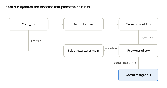
closed experimental loop · 5 steps, 1 exit

The loop repeats while the forecast is uncertain; the full target run is committed only once its forecast probability of success clears 1 − δ.

Selecting the next experiment. The next configuration is the one expected to deliver the most useful information per unit cost, where usefulness is the reduction in uncertainty about the decision in Section 7.

This is the logic of Bayesian experimental design applied to training runs. Simpler rules (run the cheapest configuration whose forecast interval still straddles the threshold) are reasonable baselines.

Correlation is not cause. A predictor can learn that a data mixture goes with higher task scores because that mixture was only ever used at larger scale. Claims that a factor X changes capability require an intervention that changes X alone, with other factors fixed and seeds randomised.

The standard error shows the practical constraint: when seed variance τ² is large relative to the effect, many replicates are needed before any causal claim is credible.

More than one objective. A change that improves task j can degrade another capability, robustness, calibration or a safety property. The optimisation is therefore constrained, not single-metric.

Here $f_{k}$ is the floor that capability or safety measure k must not fall below. The long-term objective is outcome-directed development: choosing training configurations by their forecast ability to meet explicit targets, within resource and safety constraints.

The genetic-editing analogy. A useful way to picture outcome-directed development is gene editing: if we know how changes to development parameters affect traits, we can steer the outcome instead of waiting to see what emerges. The analogy holds in one important respect and must not be pushed further. Genes influence traits through interactions with other genes, development and environment, and rarely fix every detail of the organism. Likewise, architecture, data, objectives, optimisation and compute influence learned capabilities without specifying every behaviour in closed form. The engineering analogue is capability-conditioned training: specify a target profile, estimate the effects of candidate interventions, choose a configuration, train, and validate whether the intended capability appeared.

9. Related work and the question of novelty

Forecasting downstream performance before training is an active field with working methods, so this programme does not claim the idea is new. The open question is which parts of the problem remain unsolved.

Work	What it forecasts	How	Relevance here
Kaplan et al. (2020)	Pretraining loss	Power laws in parameters, data and compute	Foundation for stage one; does not address tasks
Hoffmann et al. (2022)	Pretraining loss and compute-optimal size	Parametric law L(N, T) with irreducible term	Loss law used in Section 3
Hu et al. (2024)	Task pass rate, including code generation	PassUntil high-resolution evaluation and a task scaling law	Shows resolution is part of the method; forecast a 2.4B model before training
Ruan et al. (2024)	Downstream and agentic performance	Low-dimensional capability space fitted across about 100 public models	Found several emergent behaviours smooth and sigmoidal; observational, not controlled
Gadre et al. (2024)	Loss under over-training; average downstream error	Scaling laws over parameters and token ratio; perplexity-to-error power law	Predicted average error over 17 tasks from runs using 20 times less compute
Chen et al. (2024)	Benchmark performance of 7B and 13B models	Two-stage FLOPs to loss to performance (FLP), plus a data-mixture variant	Reported errors near 5% and 10% from samplers up to 3B; point forecasts
Schaeffer et al. (2024)	Why downstream forecasts fail	Analysis of how evaluation metrics weaken the scale-performance link	Motivates choosing metrics that preserve signal
Krajewski et al.	Downstream accuracy from training budget	Direct power law on log accuracy at fixed token-to-parameter ratio	Argues the two-stage route compounds errors; extrapolated to 6.7 times larger budgets

This literature constrains what can be claimed. Point forecasts of benchmark scores from smaller runs already work in several settings, and the data-mixture variant of FLP already addresses some transfer across mixtures.

Adjacent work that also constrains the claim. Hyperparameter optimisation already uses forecasts to allocate compute. Domhan et al. (2015) extrapolate the early part of a learning curve with a probabilistic model and stop runs that are unlikely to do well, roughly halving search time. Hyperband (Li et al.) treats configuration selection as a bandit problem, giving more resources to promising configurations and stopping the rest early. These methods select among configurations at one scale on one validation metric. The distinction this programme must demonstrate is forecasting a capability threshold, with calibrated probability, at scales and configurations beyond those observed. Work on delayed generalisation (Power et al., 2022) is relevant for the opposite reason: early learning curves can be actively misleading when a capability appears long after training accuracy saturates, which is exactly where early-stopping heuristics fail.

Candidate contributions. Each is a hypothesis to check against a systematic literature review before it is claimed as a gap.

• Threshold probabilities with calibrated uncertainty. Forecasting $\hat{π}_{j}$(κ) across repeated seeds and scoring it with Brier score and coverage, where most reported results are point errors.
• Reported extrapolation range. Measuring how forecast quality decays with the extrapolation ratio ρ and with changes to data mixture, schedule and model family.
• Joint forecasting of capability, uncertainty and cost. Treating total development cost, including failed runs and pilots, as part of the forecast target.
• Demonstrated decision value. Showing that forecast-guided experiment selection reaches a fixed capability target at lower total cost than a baseline, that is, ΔK > 0 in Section 7.

Their value depends on whether existing approaches already solve them and whether a proposed method improves on those approaches under controlled evaluation.

10. Limitations and scope

The programme forecasts learned capabilities of a trained model on defined tasks. Several things lie outside that claim, and the results must not be read as covering them.

• Prediction is not understanding. A predictor can forecast accurately without explaining the internal computation, and mechanistic insight can fail to yield accurate forecasts at scale.
• A benchmark is not general intelligence. Capabilities are multidimensional, can trade off against one another, and are measured on evaluation sets that can be incomplete, contaminated or unrepresentative.
• A base model is not a deployed agent. An agent's behaviour also depends on prompts, tools, retrieval, external software, user behaviour and environment. Intelligence, connectivity, authorisation and execution are separate variables: a model connected to a network does not thereby have permission or means to act on the systems it can reach. Forecasting the model's learned capability does not forecast the whole system.
• Factors interact. Training duration, data size and compute are coupled. One-factor-at-a-time runs diagnose effects but miss interactions; factorial designs capture them at higher cost.
• Small results may not transfer. Findings on small models and synthetic tasks may not extrapolate to frontier models, other architectures, modalities or objectives. This is tested through ρ and the transfer test, never assumed.
• Accuracy is not value. A forecast creates value only if it changes a decision for the better at lower cost than it saves (ΔK > 0).
• Dual use. A method that predicts how to develop or elicit capabilities could also make harmful capabilities cheaper to reach. Published results should consider which capabilities are studied, how methods are released, and how they interact with dangerous-capability evaluations.

11. Success and falsification criteria

The first project succeeds if, for one carefully defined task, all seven conditions below hold. Failing any one of them is itself a reportable result.

1. The capability is defined by a reproducible evaluation protocol fixed before training: $P_{j}$, $m_{j}$, $y^{*}_{j}$ and n.
2. Each predictor uses only the information in its stated set $I_{t}$, and ex ante and in-run forecasts are reported separately.
3. Every forecast is recorded and timestamped before its target run starts.
4. On $K_{\text{test}}$, the method has positive skill against every baseline in Section 6 on MAE and Brier score, at a reported extrapolation ratio ρ.
5. Forecast 90% intervals have coverage close to 0.90 across repeated seeds.
6. Any claimed saving is measured as ΔK > 0 against a baseline that reaches the same capability target, with pilot costs included.
7. The results reproduce independently from the released configurations, seeds, evaluation code and forecasts.

Predictive accuracy alone does not make the economic case. A forecast is valuable when it changes a decision and that decision improves the outcome; a method whose overhead exceeds its savings has limited practical value.

What counts against the hypothesis. The thresholds are fixed before training. For a given task, the primary hypothesis is counted as refuted if, on $K_{\text{test}}$ at the pre-registered ρ, no predictor shows positive skill over the best baseline on both MAE and Brier score, or if 90% interval coverage falls below a pre-registered floor (for example 0.75). H4 is refuted if ΔK ≤ 0. When a forecast fails, the boundary is reported as a finding; the theory is not refitted after the fact to explain every result.

12. Why I am pursuing this problem

My interest comes from resource allocation: directing limited resources toward the outcomes that create the most value.

The question began with how models develop. A trained model is not only a program that maps inputs to expected outputs; it is the product of a developmental history, including its data, training duration, compute, initialisation and the order in which it saw examples. A child-development analogy captures the intuition that broadly similar conditions need not produce identical outcomes, without implying that networks learn the way children do. Comparing models trained under controlled conditions while varying one small factor turned that intuition into an experiment. Asking whether the outcome could be predicted before training turned it into this programme.

Building companies taught me that the cost of uncertainty falls when assumptions are tested early and evidence drives the next decision. Model development has the same structure at a larger scale. A training run is an expensive computation whose outcome depends on many interacting choices; some of that outcome is already predictable, and some is not.

I want to find out how far the predictable part can be extended for task-specific capabilities and their costs. The starting proposition is testable: measurements from smaller or earlier runs may carry enough information to forecast the target capability of a more expensive run. If that holds for a defined class of tasks, the next question is whether those forecasts select better configurations and lower the cost of reaching a fixed threshold.

If the forecasts fail, the failure locates the limit: insufficient evaluation resolution, unstable scaling relationships, distribution shift, interactions between training variables, seed variance that swamps the configuration effect, or too little information in the pilots. Either outcome sharpens what is predictable in neural network development.

Conclusion

Predictive AI development asks whether the probability of reaching a capability threshold can be forecast from configuration and cheap experiments, well enough to change how compute is spent.

The core difficulty is not extrapolating a loss curve. It is that capability is a steep, noisy, resolution-limited function of loss, so forecast error concentrates exactly where decisions are made. The programme addresses this with probabilistic forecasts, held-out extrapolation, pre-recorded predictions and an explicit cost test.

The next step is concrete: fix one task and its evaluation, measure seed variance, and test whether a predictor fitted on small and early runs beats established baselines on held-out configurations. Broader claims follow from those results, not ahead of them.

References

1. Kaplan, J. et al. (2020). Scaling Laws for Neural Language Models. arXiv:2001.08361.
2. Hoffmann, J. et al. (2022). Training Compute-Optimal Large Language Models. arXiv:2203.15556.
3. Hu, S. et al. (2024). Predicting Emergent Abilities with Infinite Resolution Evaluation. ICLR 2024.
4. Ruan, Y., Maddison, C. J. and Hashimoto, T. (2024). Observational Scaling Laws and the Predictability of Language Model Performance. NeurIPS 2024.
5. Gadre, S. Y. et al. (2024). Language Models Scale Reliably with Over-Training and on Downstream Tasks. ICLR 2025.
6. Chen, Y. et al. (2024). Scaling Laws for Predicting Downstream Performance in LLMs. TMLR 2025.
7. Schaeffer, R. et al. (2024). Why Has Predicting Downstream Capabilities of Frontier AI Models with Scale Remained Elusive?. arXiv:2406.04391.
8. Krajewski, J. et al. Revisiting the Scaling Properties of Downstream Metrics in Large Language Model Training. ICLR 2026.
9. Sellam, T. et al. (2021). The MultiBERTs: BERT Reproductions for Robustness Analysis. arXiv:2106.16163.
10. Domhan, T., Springenberg, J. T. and Hutter, F. (2015). Speeding up Automatic Hyperparameter Optimization of Deep Neural Networks by Extrapolation of Learning Curves. IJCAI 2015.
11. Li, L. et al. Hyperband: A Novel Bandit-Based Approach to Hyperparameter Optimization. arXiv:1603.06560.
12. Power, A. et al. (2022). Grokking: Generalization Beyond Overfitting on Small Algorithmic Datasets. arXiv:2201.02177.